How To: Use the filter & sort feature in Excel

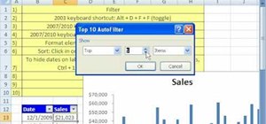
In this Software video tutorial you will learn how to use the filter & sort feature in Excel. First create a column chart on an excel sheet. In this example, it is a date and sales chart. Click alt+F1 and the chart is displayed. Then click and delete the legend and the horizontal lines. Now go back to the data set, click on a cell and click ctrl+shift+L and that will add the auto filter. ctrl+shift+L is for Excel 07. For earlier versions, see the commands listed in the video. This is a toggle. Now, to filter this, say you want to see the top five. Before that go to format > size > properties > don’t move or size with cells> close. Now click on ‘sales’ > number filters > top 10. Here you select top 5 and click OK. The video then shows you how to remove the unwanted dates and keep only the 5 required dates and how to change colors. Now to sort as per highest to lowest sales, right click on a sales cell > sort > ZtoA largest to smallest. And the data table and the chart are sorted.