How To: Automatically color alternating rows in Excel

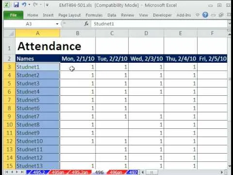
This video is a tutorial on using the Conditional Formatting function of Excel to automatically color alternating rows, which helps your eye to follow across the row. This can be done manually with the “Fill Color” button, but if you add or delete rows after applying the shading, the whole purpose is defeated.

There is an easy way to format a range of cells so that alternating rows are automatically colored, and the shading adjusts when cells are added or deleted. This works the same way in Excel 2007 and earlier versions, with slight differences.

In Excel 2003, select the cells where you want to apply the shading. Go to the “Format” menu and select “Conditional Formatting”. In the drop-down menu select “Formula Is” and type in “=mod(row(), 2)”. (This formula works by combining two different functions, and is explained in detail at the end of the video.) When the conditions of the formatting are true, the formatting is applied. Click on “Format” and change the background pattern, click OK, and the alternating rows are now colored. The formatting can easily be changed or removed, and you can also apply it to columns rather than rows.

In Excel 2007, select the range of cells, making sure you are in the “Home” menu. The “Conditional Formatting” command is in the “Styles” section. Select “New Rule”, then select “Use a formula to determine which cells to format”. In the formula box type the formula as before, select your formatting and click OK. You can go back to the “Conditional Formatting” command if you want to clear the formatting from selected cells or the entire sheet, or you can change the formatting or the formula with the “Manage Rules” command.