How To: Make a dynamic named range in Excel (left to right)

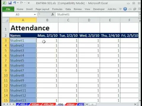
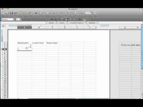
Teach Excel describes how to create a dynamically updating named range that goes from left to right using Excel. First, you define the named range by highlighting the cells containing numbers in a certain row. In the name box to the left of the formula bar, type the name of the data. In this example, the numbers correspond to sales, so type "sales." To check if the named range works, click on an empty cell and enter =sum(sales). That should return the sum of the highlighted cells. However, as you add more data to the row, the total will not update because it is not dynamic. To create a dynamic named range, choose a blank cell and type =offset(). Within the parentheses, add the following values separated by commas: the cell of the first number in your list (ex. B2), the reference row (0), the reference column (0), the row height (1), and the row width. For the row width, type count( and then select the entire row by click in the row number. Close the parentheses and the row width should look something like this: count(2:2). The entire formula should look similar to this: =offset(B2, 0, 0, 1, count(2:2)). Press enter, highlight the formula, copy it, and hit Ctrl+F3 for the Name Manager window. Then click the sales reference and delete the formula in the "Refers to:" box. Paste the formula you copied into the box and click the checkbox. Close the window and the named range should be dynamic. Test this by adding data to the end of your row and observing the changes to the total.